The following is my report from the Predicting Mortgage Approvals April 2019 Capstone Project from the Microsoft Professional Program in Data Science.  The findings provided below are representative ONLY of the training and test datasets that were provided for the project and not of all mortgage approvals in the US.  Indeed as mentioned in the report, Exploratory Data Analysis revealed that the datasets did not provide a full picture of mortgages in the United States, but only a portion of loans over some undetermined amount of years that were representative of loans from applicants in areas with incomes at or lower than the MSA-MD median.  By definition of median, a more representative sample of loans would have included loans from applicants in areas with incomes higher than the MSA-MD median.

Executive Summary

This document presents the analysis of government data used with regards to mortgage approvals in the United States. The goal of the project is to predict mortgage approvals from the data. The analysis is based on 500,000 observations of loan applications. Each of these observations contained data on each loan application including three categorical features describing the location of the property within the country (Property Location Features), seven features regarding the loan itself (Loan Information Features), five describing demographic information about the applicant (Applicant Information Features), and finally Census Information; six features which describe demographic and property characteristics of the geographic area where the property being mortgaged is located. Finally, the index and target variable were included.

After examining summary and descriptive statistics and exploring the data through visualizations, further manipulation of the data was needed to hone-in on the key relationships. Additional features were developed based on the original features to better capture the relationships. Once these were determined the model was developed to provide the most predictive result.

The following conclusions were found:

While many of the features in the dataset contributed to model’s ability to predict mortgage acceptance, there were five significant features:

• Lender – a categorical feature with no ordering indicating which of the lenders was the authority in approving or denying this loan. In this dataset there were over 6,000 lenders.
• Applicant Income – a numeric feature as name describes recorded in thousands of dollars.
• Loan Purpose – a categorical feature indicating whether the purpose of the loan or application was for home purchase, home improvement, or refinancing.
• Loan Amount – a numeric feature representing the size of the requested loan in thousands of dollars.
• LC – a categorical feature created to group the lenders into five categories based on the frequency of loans they service in order to determine if the size of lender makes a difference in the acceptance rate. The resulting categories from highest frequency to least: Mega, Large, Mid, Small and Mini.

Exploratory Data Analysis

Numeric Features

There are 8 numeric features on the data set.

Loan Information Feature

• loan_amount: the size of the requested loan in thousands of dollars

Applicant Information Feature

• applicant_income: as described in thousands of dollars

 Census Information Features:

• population: total population in the (approximately) 4000-person Census tract.
• minority_population_pct: the percent of minority population of the tract.
• ffiecmedian_family_income: the annually adjust FFIEC Median Family Income of the MSA-MD in which the tract is located.
• tract_to_msa_md_income_pct: the percent of the tract family income to the MSA-MD median family income.
• number_of_owner_occupied_units: number of dwellings, including condominiums, that are lived in by the owner.
• number_of_1_to_4_family_units: number of dwelling that are built to house fewer than 5 families.

Summary Statistics were first gathered on the numeric features to determine count, unique count, missing values, minimum, maximum, mean, mean deviation, 1^st quartile, median, 3^rd quartile, mode, range, variance and standard deviation:

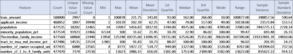
There are some large ranges in the data. It’s important to be cognizant of unit of measure when looking at the table. The range for ffiecmedian_family_income is in dollars, which may be reasonable, while the ranges for loan_amount and applicant income are in thousands of dollars, indicating there are some outliers.

Additional columns were created to capture relationships between the data. Finding a way to address the cost of living differences across the United States was hypothesized to be predictive given the occurrence of Property Location and Census features in the data.

Calculated columns were created for:

• loan_to_tract_median: loan amount divided by ffiec median family income adjusted for differences in unit of measure
• app_inc_to_tract_median: applicant income divided by ffiec median family income adjusted for difference in unit of measure.

Both of these measures were in a secondary tier of predictors for the model.

To be noted were some oddities in the census data.

Inspection of the data led to the finding that FFIEC median family income would change for rows with the same state, county and MSA/MD, indicating either errors or more likely that the data spanned a number of years. This may muddy efforts of trying to pick up cost of living differences among the data.

The tract_to_msa_md_income_pct could have been a telling predictor in terms of cost of living. However further examination of the data showed that there was no instance in the training or test data that was over 100% though there should have been if the data sets were representative of all loans. (People living in tracts with median incomes above the MSA/MD median income in which the tracts are located apply for loans too.) So this tells us that the data sets provided were for a portion of loans in which the tract median income is at or below the MSA/MD median income.

Categorical Features

There are 13 categorical features in the dataset besides the label. They are as follows:

Property Location Features

• msa_md: this feature represents an ID for the Metropolitan Statistical Area/Metropolitan Division (MSA-MD) where the property may be located. Missing values are indicated with a -1.
• county_code: this feature represents an ID for the county in which the property is located. Missing values are indicated with a -1.
• state_code: this feature represents an ID for the state in which the property is located.

Loan Information Features

• lender: this feature represents the ID of the lender that was the approving authority of the loan.
• loan_type: indicates whether the loan was Conventional, FHA-insured, VA guaranteed, Farm Service Agency or Rural Housing Service
• property_type: indicates whether the loan was for a one-to-four-family dwelling (non-manufactured), manufactured housing or multifamily.
• loan_purpose: indicates whether the purpose of the loan was for home purchase, home improvement or refinancing
• occupancy: indicates whether the property in the loan application will be owner-occupied, not owner-occupied or N/A.
• preapproval: whether pre-approval was requested before the loan application was placed. Values include pre-approval was requested, pre-approval was not requested or N/A

Applicant Information Features

• applicant_ethnicity: Hispanic or Latino, Not Hispanic or Latino, Not Provided, N/A and No Co-applicant
• applicant_race: American Indian r Alaska Native, Asian, Black or African American, Native Hawaiian or other Pacific Islander, White, Not Provided, N/A, No Co-applicant
• applicant_sex: Male, Female, Not Provided or N/A
• co-applicant: true or false

Additional categorical columns were created to delve into relationships in the data and potentially reduce the noise in the model. There are 6111 lenders in the data set. To look at them in a bar chart is fruitless. They needed to be grouped in some other way. Grouping them by rate of acceptance would be great but only works if the lenders are the same in the test data. However this was not the case. So frequency was used to bin lenders into categories by the volume of loans they oversee in the dataset as Mega, Large, Mid, Small and Mini. The categories by acceptance rates can be seen here:

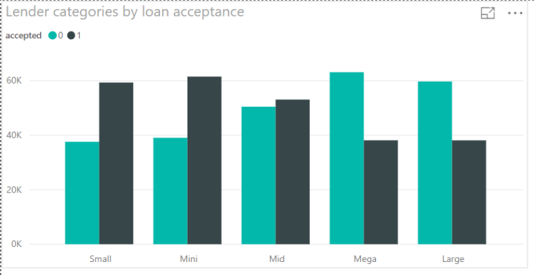
Clearly there is a difference in the rates of acceptance by category. The Mega and Large lenders have more denials, while the Small and Mini lenders have more acceptances. As such, this feature consistently showed up as a top 5 contributor to the accuracy of the model.

The same thought process was applied to the Property Location features.

The following chart shows state_codes by acceptance.

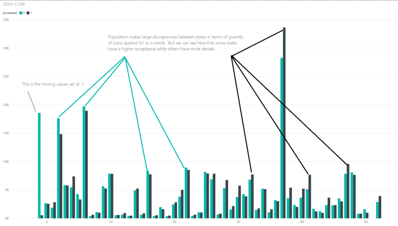
The charts for counties and msa_mds are largely illegible due to the quantity of categories. The same process to bin the lenders was carried out with these features. The missing values in these features were respected because in examining the data it was clear that missing a value in each of these features was a strong indicator that the loan would be denied. The frequency of loans per code were counted up and then the various codes were assigned to groups based on their frequency (High, Mid, Low) and the -1s were coded to NP for “not provided.”

The following graphs show the resulting new category features and their frequencies by acceptance.

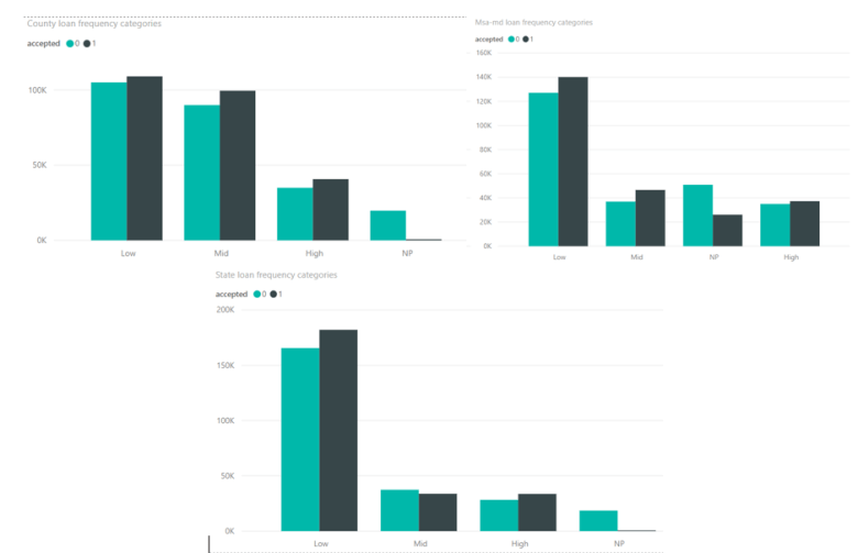
For State and MSA-MD codes there are a higher number of low frequency States and MSA-MDs, but from a frequency perspective there is not too much variation between acceptance and denial among the categories (with the exception of the NPs). You can see the large rate of denials where there are missing values. This frequency binning for each of these features did not prove to be as predictive as the original features they were produced from.

Key Findings

Research revealed some important aspects of these features. MSA-MDs do not cover the entire country. Therefore, there may be instances in the data where the code is not missing or left out, but simply does not exist for the property.

The county codes are not unique in the dataset. For example, multiple instances of county_code 243 can be found in state_codes 1 and 10. Additionally further examination of the Geocoding map shows that an MSA-MD can encompass multiple counties. So the county is the smallest geographical area of these property locations, though there are far more unique MSA_MD codes. This, again, is because the county codes are not unique.

In reality there are 3,140 counties in the United States whereas there are only 318 in the dataset. To arrive at a true county code, some models were run with a concatenated state_code and county code, separated by a comma to determine if the true county codes were significant in predicting the model. This created 3,194 true counties, but binning was not introduced. On its own (without binning), the true county code did not appear to be helpful, though with the state and county codes merged into the concatenated column, it did push the county category code up higher in the ranks of contributing to the predictiveness of the model. This leads me to deduct that however the county_codes were applied to the training data for this competition had some form of relationship to the acceptance rates.

Analysis of the bar charts of the rest of the categorical features showed the following (charts shown for significant relationships):

• Not Hispanic or Latino is by far the most common entry in applicant_ethnicity
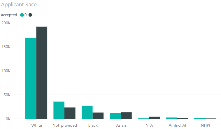
• White is the most common entry in applicant_race.
• Within applicant_race acceptance rates are higher for Whites and Asians, while lower for Blacks, American Indian/Alaska Natives and Native Hawaiian/Pacific Islander

• Males apply for more loans than females and have a higher rate of acceptance than females whose denial rate is higher.
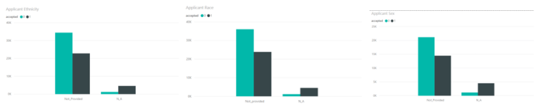
• The small frequencies of Not Provided and N/A among applicant_ethnicity, applicant_race and applicant_sex would suggest that they should be binned together. However, this hurt model performance. This occurred because across these features, the Not Provided categories had a higher rate of denial, while the N/A categories provided a higher acceptance rate as can be seen here.

• There’s a higher rate of acceptance if there is a co-applicant, but there are more loans without co-applicants.
• 1 to 4 family dwelling was by far the most common property type and had a higher level of acceptance than denial.
• Conventional was by far the most common loan type, but the categories were well balanced between acceptance and denial.
• Within loan_purpose, Re-financing was the most common reason followed not far behind by Home Purchase. Acceptances were more likely in Purchases while denials were more likely in Re-financing and Home Improvement loans.

• Owner-occupied was by far the most common occurrence in the occupancy feature. The rates of loan acceptance to denial were even amongst the categories.
• The vast majority of pre-approvals were N/A and those were fairly evenly balanced between accepted and denied. The lowest frequency category of Requested Pre-approval had a higher denial rate, while the low frequency category of Not Requested Pre-approval had a higher acceptance rate.

Correlations and Apparent Relationships

We are predicting accepted loans. The accepted label is either 0, meaning the loan is denied, or 1, the loan is accepted. It is important to determine if the data set is balanced on the label or if an adjustment needs to be made to the data set to correct for class imbalance. As it turns out, this data set is balanced. Half of the loans are accepted and half denied in the dataset.

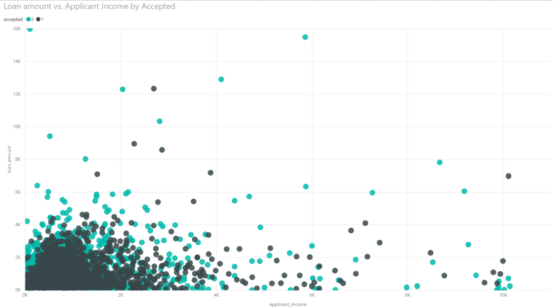
The large dataset proved tricky when viewing the various visualizations used to find relationships among the data. In particular, scatterplots had a great deal of concentrated density within a small range while data points exist in a much larger range which can be seen in the following charts.

I used Power BI for initial visualizations so that I could filter through the density. One thing that can be seen clearly from this graph is that in general, there are more acceptances amongst loans of lower amount. Additionally, the outliers can be viewed here.

Azure ML Studio and Jupyter Notebook were used to create the model and further explore the data.

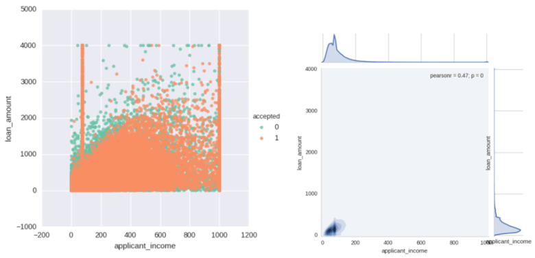
The following plots show the concentrated density and the long tails of loan_amount and applicant_income AFTER the outliers were highly clipped back to threshold and missing values of applicant income were changed to median (PCA and MICE produced some negative values). The bulk of loans are highly concentrated into a small window of loan amount and applicant income. Observe in the density plot on the right how the tails for applicant income start around 200, but on the scatter plot, values of applicant income in the scatterplot on the left are still very dense beyond this point. This is due to the large size of the data set.

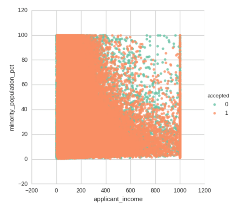
Besides the relationship between applicant income and loan amount, there aren’t very many clear relationships between the rest of the numerical features other than a pocket of more denials where high applicant income and high minority_population_pct met.

Classification of Mortgages Based on Acceptance

The analysis of the features led to a reiterative process to develop the most predictive classification model to determine whether a loan would be accepted (score of 1) or denied (score of 0).

Ultimately the following 19 features were used to test the model in order of importance to the accuracy statistic based on the Permutation Feature Importance module in Azure Machine Learning Studio:

1. Lender
2. Applicant Income
3. Loan purpose
4. Lender Category
5. Loan amount
6. County Category
7. Loan type
8. Property type
9. Applicant race
10. Loan to tract median
11. Applicant income to tract income
12. MSA-MD
13. Occupancy
14. Applicant ethnicity
15. State category
16. Co-applicant
17. Pre-approval
18. Minority population percent
19. Applicant sex

The data was split 70% to train and 30% to test. Through Cross Validation, the Two-Class Boosted Decision Tree algorithm, tuned for hyperparameters was found to yield the best results:

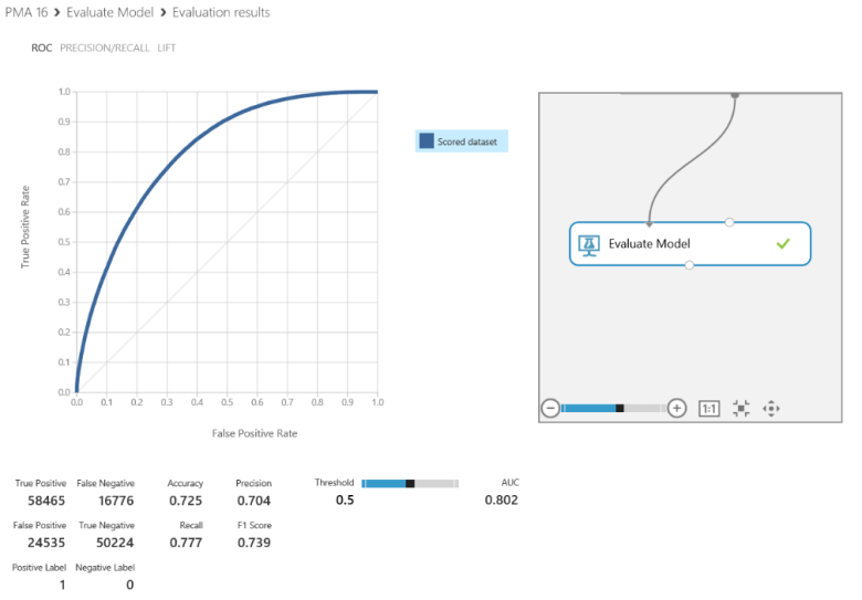
The true and false positive and negative rates can be examined above along with the ROC curve as well as their corresponding Accuracy, Precision, Recall and F1 Score. The diagonal line in the chart represents a random guess while the closer the curve moves toward the left and top axes indicates a higher rate of accuracy.

Accuracy was the driving statistic of this project. Seventy-two and a half percent accuracy was the highest reached amongst the iterations of the models.

Conclusion

This analysis has shown that mortgages can be reasonably well predicted verses a random guess from government data. The most important features in the predictive model are lender and it’s corresponding lender frequency category, loan amount, application amount and loan purpose. Secondarily, a number of loan information, and property location features contributed to its accuracy including county frequency category, loan type, applicant race, loan to tract median income, and applicant income to tract median income.

Recommendations

Ethical considerations

The goal of this competition and this portion of the capstone project was to achieve the highest level of Accuracy that we could. In order to do that, applicant demographic data was used. Ethical considerations must be addressed when dealing with this type of data.

In the case of predicting mortgage acceptance, using demographical data can be helpful to determine if lenders or even certain geographical regions of the country are discriminating against minorities. The data used in this project shows some evidence of that. These insights can be used to create policies that protect minorities.

It should be noted that removing the sensitive demographic data from the model yields the following result. We can see a lower accuracy rating.

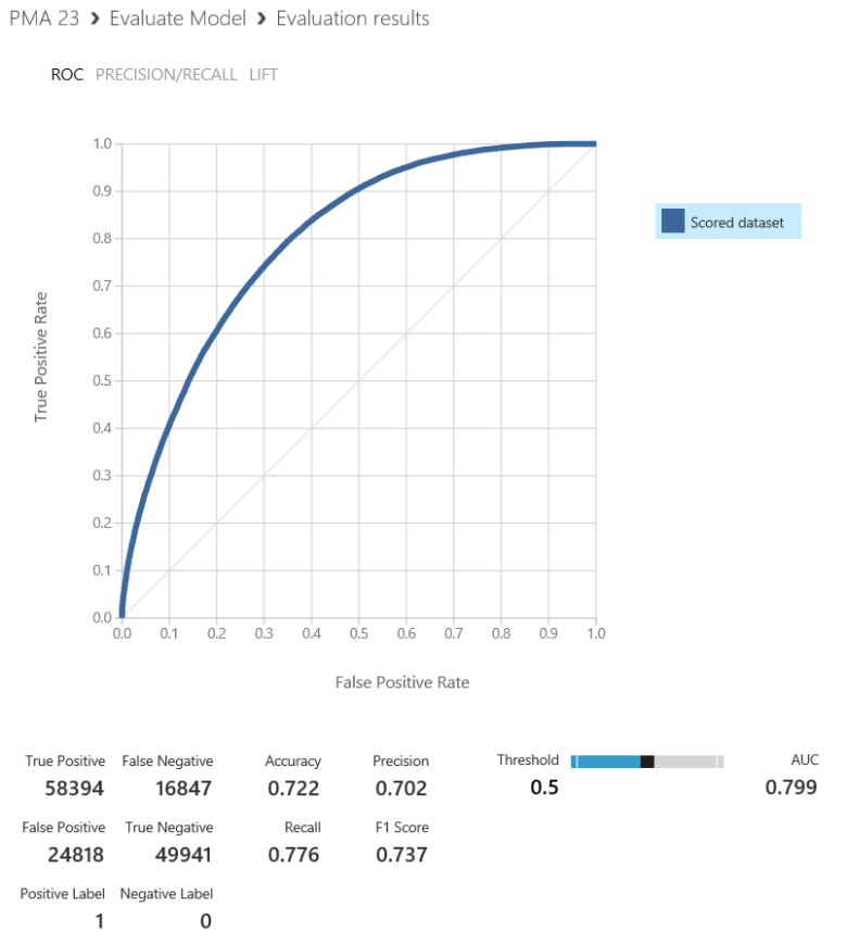
While the data provides greater accuracy, the use of it needs to be carefully administered so that it is being used to promote solutions to discrepancies between demographic categories and not used as a means of risk protection for lenders to deny loans. This would create a negative feedback loop that will further exacerbate the discrepancies found here.

How the model could be improved

• Run an ensemble method of classifiers. This method was unable to be completed at the writing of this report.
• The process of writing the report has lead to further thoughts on ways to manipulate the data. I kept notes while I was working on my hypotheses, thought process and visualizations, but the organization of the report has realigned things. I think writing the report post-initial exploration, feature selection and algorithm determination, but pre-tweaking would have allowed further substantive development of the model and its accuracy.